 INNO fibre optic temperature sensors ,temperature monitoring systems.
- MRI systems require precise temperature control for superconducting magnets, gradient coils, and RF components to ensure optimal performance
- Gradient coil overheating is the most common temperature-related issue, accounting for 35-40% of MRI thermal failures
- Traditional temperature sensors containing metallic components are incompatible with MRI’s strong magnetic fields (1.5T-7T)
- Fluorescent fiber optic temperature sensors provide MRI-compatible monitoring with ±1°C accuracy from -40°C to +260°C
- One fiber optic cable measures one specific hotspot; single transmitters support 1-64 independent channels
- Proper temperature monitoring extends MRI system lifespan by 15-25% and reduces unplanned downtime by 40-60%
- Beyond MRI, fiber optic sensors monitor CT scanners, PET systems, linear accelerators, and laboratory equipment
Table of Contents
- What is Magnetic Resonance Imaging (MRI) System
- How MRI Systems Work
- Primary Functions of MRI Equipment
- MRI Application Range
- MRI System Maintenance and Service
- Superconducting MRI vs Permanent Magnet MRI
- Common MRI Failures and Issues
- MRI Temperature Abnormality Solutions
- MRI Monitoring Equipment Components
- MRI Temperature Monitoring Solutions
- Temperature Sensor Comparison: Why Fluorescent Fiber Optic Sensors
- Medical Equipment Overview
- Fiber Optic Temperature Monitoring for Equipment Hotspot Detection
- Frequently Asked Questions
1. What is Magnetic Resonance Imaging (MRI) System

Magnetic Resonance Imaging (MRI) is an advanced medical diagnostic technology that uses powerful magnetic fields, radio frequency pulses, and sophisticated computer processing to generate detailed anatomical images of internal body structures. Unlike X-ray or CT scanning, MRI systems produce images without ionizing radiation, making them particularly valuable for repeated examinations and pediatric applications.
The fundamental principle involves aligning hydrogen atoms in the body using a strong magnetic field, then disturbing this alignment with radiofrequency energy. As the atoms return to equilibrium, they emit signals that are detected and processed into high-resolution images showing exceptional soft tissue contrast.
A complete MRI scanner consists of several integrated subsystems working in precise coordination:
Primary Magnet System
The superconducting magnet forms the core of most clinical MRI systems, generating static magnetic fields ranging from 1.5 Tesla to 7 Tesla—30,000 to 140,000 times stronger than Earth’s magnetic field. These magnets use niobium-titanium wire coils cooled to -269°C (4 Kelvin) with liquid helium, maintaining superconductivity with zero electrical resistance. The magnet operates continuously, 24 hours per day, for years without interruption.
Gradient Coil Assembly
Gradient coils create precisely controlled variations in the magnetic field, enabling spatial encoding of MR signals. These electromagnetic coils switch rapidly during scanning—up to 200 times per second—generating the characteristic knocking sounds during MRI examinations. This rapid switching produces significant heat, making gradient coil temperature monitoring critical for system reliability.
Radiofrequency (RF) System
RF coils transmit radiofrequency pulses to excite hydrogen atoms and receive the resulting MR signals. Transmit coils require high-power amplifiers generating several kilowatts, while sensitive receive coils detect signals measured in microvolts. Both components generate heat requiring active cooling and temperature monitoring.
Cooling Infrastructure
Multiple cooling systems maintain operational temperatures: liquid helium cryostats preserve superconductivity in the main magnet, chilled water circuits cool gradient coils and RF amplifiers, and facility HVAC systems maintain proper room temperature (18-22°C) and humidity (30-60% RH).
Field Strength Classifications
MRI scanners are categorized by magnetic field strength:
- Low-field systems (0.2-0.5T) – Open MRI designs, primarily permanent magnets, limited imaging capabilities but excellent patient comfort
- Mid-field systems (1.0-1.5T) – Workhorse clinical scanners balancing image quality, operating costs, and versatility
- High-field systems (3.0T) – Advanced clinical imaging with superior signal-to-noise ratio, faster scanning, specialized applications
- Ultra-high-field systems (7.0T and above) – Research applications, exceptional resolution, regulatory approval for limited clinical use
Modern MRI technology continues evolving with wider bores (70cm) improving patient comfort, higher field strengths enhancing image quality, and artificial intelligence accelerating image acquisition and interpretation.
2. How MRI Systems Work
The MRI imaging process exploits fundamental quantum mechanical properties of atomic nuclei, specifically hydrogen protons abundant in water and fat molecules comprising human tissue.
Magnetic Field Alignment
When a patient enters the MRI scanner’s strong magnetic field, hydrogen protons throughout the body align either parallel or anti-parallel to the field direction. A slight majority align parallel, creating a net magnetic moment that forms the basis for MR signal generation. This alignment occurs within milliseconds and persists as long as the magnetic field remains constant.
Radiofrequency Excitation
The RF system transmits precisely tuned radiofrequency pulses (typically 63.9 MHz for 1.5T systems, 127.8 MHz for 3T) that resonate with hydrogen protons at their Larmor frequency. This energy absorption tips the protons away from their aligned state, storing energy in the nuclear magnetic moment like winding a spring.
Signal Emission and Detection
When the RF pulse ends, excited protons relax back to equilibrium alignment, releasing absorbed energy as radiofrequency signals. Receiver coils detect these tiny signals—often just microvolts in amplitude—and amplify them for processing. Two relaxation processes occur simultaneously:
T1 Relaxation (Spin-Lattice Relaxation)
Protons realign with the main magnetic field, releasing energy to surrounding tissue. Different tissues exhibit characteristic T1 relaxation times ranging from 200-2000 milliseconds, providing tissue contrast.
T2 Relaxation (Spin-Spin Relaxation)
Proton magnetic moments dephase due to local field variations, causing signal decay. T2 times range from 30-200 milliseconds, creating different contrast mechanisms.
Spatial Encoding with Gradient Fields
Gradient coils apply precisely controlled magnetic field variations along three axes (X, Y, Z), causing protons at different locations to resonate at slightly different frequencies. This frequency encoding combined with phase encoding allows the MRI computer to determine signal origin and construct spatial images.
Image Reconstruction
Sophisticated computer algorithms—primarily Fast Fourier Transform (FFT)—convert received frequency and phase data into anatomical images. A typical MRI scan acquires millions of data points over several minutes, reconstructing images with voxel resolutions approaching 1 cubic millimeter.
Pulse Sequence Programming
MRI sequences combine specific RF pulses, gradient patterns, and timing parameters to emphasize different tissue properties:
- T1-weighted imaging – Excellent anatomical detail, fat appears bright, fluid appears dark
- T2-weighted imaging – Superior pathology detection, fluid appears bright, highlighting edema and inflammation
- Proton density imaging – Tissue contrast based purely on hydrogen concentration
- Diffusion-weighted imaging – Detects water molecule movement, critical for stroke diagnosis
- Functional MRI (fMRI) – Measures brain activity through blood oxygenation changes
3. Primary Functions of MRI Equipment
MRI systems serve multiple critical roles in modern healthcare, extending beyond simple anatomical imaging to functional assessment and therapeutic guidance.
Soft Tissue Visualization
The unparalleled soft tissue contrast of magnetic resonance imaging enables visualization of structures poorly seen by other modalities. Brain white matter versus gray matter differentiation, meniscal tears in knee joints, intervertebral disc degeneration, and liver lesion characterization exemplify MRI’s superior soft tissue discrimination.
Disease Diagnosis and Staging
MRI scanning provides definitive diagnosis for numerous conditions:
- Neurological disorders – Multiple sclerosis plaques, brain tumors, stroke evolution, spinal cord compression
- Musculoskeletal injuries – Ligament tears, cartilage damage, bone marrow edema, stress fractures
- Cardiovascular disease – Myocardial viability, cardiac chamber volumes, congenital heart defects, aortic aneurysms
- Oncology applications – Tumor detection, treatment response assessment, metastasis screening, radiation therapy planning
- Abdominal pathology – Liver lesions, pancreatic masses, renal cysts, prostate cancer
Functional and Physiological Assessment
Advanced MRI techniques measure physiological processes beyond static anatomy:
Functional MRI (fMRI)
Detects brain activity by measuring blood oxygenation changes during cognitive tasks, mapping eloquent cortex before brain surgery, and investigating neurological disorders.
MR Spectroscopy (MRS)
Analyzes tissue biochemistry by detecting metabolite concentrations, differentiating tumor recurrence from radiation necrosis, and assessing metabolic disorders.
Diffusion Tensor Imaging (DTI)
Maps white matter tract connectivity in the brain, guiding neurosurgical approaches and evaluating traumatic brain injury.
MR Angiography (MRA)
Visualizes blood vessels without contrast injection, screening for aneurysms, stenosis, and vascular malformations.
Treatment Guidance and Monitoring
Interventional MRI guides minimally invasive procedures including tumor biopsies, therapeutic injections, and thermal ablations. Real-time MRI temperature imaging monitors ablation procedures, ensuring complete tumor destruction while protecting adjacent normal tissue.
4. MRI Application Range
Magnetic resonance imaging applications span diverse medical specialties, research institutions, and increasingly veterinary medicine, with each domain requiring specific technical configurations and monitoring approaches.
| Application Sector | Typical Field Strength | Common Examinations | Key Advantages | Temperature Monitoring Priority |
|---|---|---|---|---|
| Neurology | 1.5T – 3.0T | Brain tumors, stroke, MS, epilepsy | Superior gray/white matter contrast | High (long scan times) |
| Orthopedics | 1.5T – 3.0T | Joint injuries, spine, sports medicine | Cartilage and ligament visualization | Medium (moderate duty cycle) |
| Cardiology | 1.5T – 3.0T | Myocardial viability, CHD, cardiomyopathy | Functional cardiac assessment | High (cardiac gating, long scans) |
| Oncology | 1.5T – 3.0T | Tumor staging, metastasis, response | Whole-body imaging capability | High (extended protocols) |
| Pediatrics | 1.5T – 3.0T | Congenital abnormalities, tumors | No ionizing radiation | Medium (shorter scans typical) |
| Breast Imaging | 1.5T – 3.0T | Cancer detection, high-risk screening | Superior sensitivity in dense tissue | Medium (dedicated breast coils) |
| Research Institutions | 3.0T – 7.0T+ | fMRI, spectroscopy, methodology | Maximum SNR and resolution | Critical (ultra-high duty cycles) |
| Veterinary Medicine | 0.5T – 1.5T | Equine, canine, exotic animals | Non-invasive soft tissue imaging | Medium (variable case complexity) |
| Prostate Imaging | 3.0T preferred | Cancer detection, biopsy guidance | Multi-parametric protocols | High (complex sequences) |
| Abdominal Imaging | 1.5T – 3.0T | Liver, pancreas, kidney pathology | Contrast-free tissue characterization | Medium (breath-hold techniques) |
Clinical Hospital Installations
General hospitals typically operate 1.5T MRI scanners as primary workhorses, handling 15-25 patients daily across all clinical indications. Large academic medical centers deploy multiple systems including 3.0T units for specialized neurological and musculoskeletal imaging, performing 30-50 scans daily per machine.
Specialized Imaging Centers
Outpatient MRI facilities focus on high-volume orthopedic and spine imaging, often utilizing wide-bore 1.5T systems accommodating larger patients and those with claustrophobia. Some centers deploy open MRI designs (permanent magnets or low-field superconducting) prioritizing patient comfort over ultimate image quality.
Research and Academic Institutions
University research programs operate ultra-high-field MRI systems (7T and above) exploring brain connectivity, metabolic imaging, and methodological development. These installations demand stringent temperature monitoring due to extended scanning protocols and experimental sequences pushing hardware limits.
Interventional and Surgical Suites
Intraoperative MRI systems integrated into neurosurgical operating rooms enable real-time imaging during tumor resections, guiding complete removal while preserving critical brain structures. These systems experience intermittent but intensive use, creating thermal cycling stress on gradient and RF components.
Mobile MRI Services
Trailer-mounted MRI scanners provide imaging services to underserved areas or supplement hospital capacity during peak demand. These systems face additional environmental challenges including temperature extremes, vibration during transport, and varying power quality requiring robust monitoring systems.
Veterinary Applications
Specialty veterinary hospitals deploy MRI systems for companion animals and livestock, particularly valuable for neurological conditions in horses and dogs. Lower field strengths (0.5-1.5T) often suffice given smaller patient sizes, but scanning protocols may extend for hours under general anesthesia.
5. MRI System Maintenance and Service
Proper MRI maintenance ensures consistent image quality, maximizes system uptime, and protects the substantial investment—often $1-3 million for the scanner plus $500K-1M for facility infrastructure. Maintenance strategies combine manufacturer-recommended schedules with condition-based monitoring.
Daily Operational Checks
MRI technologists perform brief system verification before patient scanning begins:
- Helium level inspection – Visual check of cryogen gauge, verifying >60% capacity (critical level ~40%)
- Gradient coil performance – Phantom scan verifying image quality and geometric accuracy within specifications
- Cooling system status – Confirm chilled water flow rates (typically 15-25 liters/minute) and temperatures (10-15°C supply)
- Room environmental conditions – Temperature 18-22°C, relative humidity 30-60%, ensuring stable operating environment
- RF system function – Transmit power calibration and receive coil operation verification
These checks consume 15-20 minutes but prevent costly downtime from preventable issues.
Weekly and Monthly Inspections
Preventive maintenance on weekly cycles includes:
- Detailed phantom imaging with quantitative analysis of signal-to-noise ratio, geometric accuracy, and image uniformity
- Cooling system filter inspection and cleaning
- Gradient amplifier status review including fault logs and temperature excursions
- RF amplifier performance verification and cooling check
- Patient table mechanical operation and weight capacity testing
Monthly tasks add comprehensive electrical safety testing, emergency stop function verification, and quench pipe inspection ensuring helium venting pathway remains unobstructed.
Quarterly Preventive Maintenance
Manufacturer-certified engineers perform detailed MRI service every 3 months:
- Gradient system evaluation – Detailed electrical testing of gradient amplifiers, coil resistance measurements, and cooling system performance under maximum load conditions
- RF system calibration – Transmit power optimization, receiver gain calibration, and coil quality factor measurements
- Cryogen system inspection – Helium boil-off rate assessment, cold head operation verification, pressure relief system testing
- Mechanical system service – Patient table lubrication, positioning accuracy verification, bore lighting and ventilation check
- Computer system maintenance – Software updates, database optimization, backup verification, disk space management
Quarterly service typically requires 4-8 hours of system downtime scheduled during off-peak periods.
Annual Major Service
Comprehensive annual maintenance includes all quarterly items plus:
- Complete gradient coil performance testing including eddy current characterization and temperature rise measurements
- RF coil inventory inspection with connector integrity and element function verification
- Magnet shimming optimization restoring field homogeneity after drift from ferromagnetic object exposure
- Cooling system complete service including heat exchanger cleaning, fluid analysis and replacement, pump inspection
- Electrical safety testing per IEC 60601 standards including leakage current and ground integrity
- Image quality phantom scanning with comprehensive analysis against baseline performance
Helium Management
Liquid helium maintains the superconducting magnet at 4 Kelvin (-269°C). Modern MRI systems use zero-boil-off cryostats with two-stage cold heads compressing and re-liquefying evaporated helium, reducing boil-off rates to 0.1-0.5 liters per day from historical rates of 2-5 liters daily. Despite this efficiency, helium refills remain necessary every 3-5 years, costing $20,000-40,000 per fill depending on market conditions.
Critical helium monitoring includes:
- Continuous liquid level monitoring with alarms at 50% (refill planning) and 30% (urgent refill required)
- Cold head operation verification ensuring compressor runs properly and achieves target temperatures
- Pressure monitoring confirming system maintains 1-3 psi above atmospheric
Temperature Monitoring Integration
Gradient coil temperature monitoring provides early warning of cooling system degradation, sequence programming errors causing excessive duty cycles, or mechanical issues creating hotspots. Continuous monitoring enables predictive maintenance scheduling before thermal damage occurs.
Maintenance Documentation
Comprehensive service records document all maintenance activities, component replacements, performance measurements, and system modifications. This data supports warranty claims, regulatory compliance (FDA, state health departments), and predictive analytics identifying degradation trends before failures.
6. Superconducting MRI vs Permanent Magnet MRI
The fundamental choice between superconducting MRI and permanent magnet MRI systems involves balancing image quality requirements, budget constraints, facility limitations, and clinical applications.
| Comparison Factor | Superconducting MRI | Permanent Magnet MRI |
|---|---|---|
| Magnet Technology | Niobium-titanium coils at -269°C | Rare-earth permanent magnets (room temp) |
| Field Strength Range | 1.0T – 7.0T (clinical: 1.5T, 3.0T) | 0.2T – 0.7T (typical: 0.3T – 0.4T) |
| Field Orientation | Horizontal (patient lies along field) | Vertical (patient sits/stands in field) |
| Bore Configuration | Cylindrical tunnel (60-70cm diameter) | Open sides (C-arm or four-post design) |
| Image Quality (SNR) | Excellent to outstanding | Good for limited applications |
| Scan Time | 5-30 minutes typical | 15-45 minutes typical |
| Spatial Resolution | Sub-millimeter achievable | 1-2mm practical limit |
| Clinical Applications | Full range of indications | Extremities, spine, limited body imaging |
| Cooling Requirements | Liquid helium + chilled water systems | Room temperature (HVAC only) |
| Helium Dependence | Critical (refill every 3-5 years) | None (no cryogens required) |
| Power Consumption | 30-50 kW (includes cooling) | 15-25 kW |
| System Weight | 5,000-15,000 kg | 8,000-25,000 kg (heavier magnets needed) |
| Fringe Field | Extensive (5 gauss: 5-10m radius) | Limited (5 gauss: 1-3m radius) |
| Site Preparation Cost | $300K-800K (RF shielding, HVAC, power) | $100K-300K (simpler requirements) |
| Equipment Cost | $1.0M-3.0M+ (field strength dependent) | $400K-900K |
| Annual Operating Cost | $150K-300K (service, helium, utilities) | $80K-150K (service, utilities) |
| Patient Comfort | Claustrophobia common (15-20% patients) | Excellent (open design reduces anxiety) |
| Patient Accessibility | Limited (weight limits 150-250kg) | Good (accommodates larger patients) |
| Interventional Use | Challenging (access limitations) | Excellent (physician access during scanning) |
| Field Stability | Exceptional (drift <0.1 ppm/hour) | Good (temperature dependent, 1-5 ppm/hour) |
| Maintenance Complexity | High (specialized cryogenic service) | Moderate (conventional systems) |
| Quench Risk | Present (rare but expensive event) | None (no superconducting elements) |
| Temperature Monitoring Needs | Critical (gradient coils, RF, cryogenics) | Moderate (gradient coils, RF amplifiers) |
Image Quality and Clinical Performance
The fundamental advantage of superconducting MRI systems lies in superior signal-to-noise ratio (SNR) directly proportional to field strength. A 3.0T system provides approximately twice the SNR of a 1.5T system, enabling faster scanning, higher resolution, or both. This SNR advantage proves critical for neurological imaging, cardiac MRI, and advanced techniques like diffusion tensor imaging.
Permanent magnet MRI at 0.3-0.4T generates adequate images for basic musculoskeletal studies—extremity joints, spine—but struggles with abdominal imaging due to motion artifacts and low SNR. Brain imaging quality remains diagnostic for many indications but lacks the detail necessary for subtle white matter lesions or small structural abnormalities.
Economic Considerations
Total ownership cost analysis over 10 years reveals different value propositions:
Superconducting MRI (1.5T system example):
- Equipment: $1,500,000
- Site preparation: $500,000
- Annual service contracts: $120,000 × 10 = $1,200,000
- Helium refills (2 times): $70,000
- Utilities: $40,000 × 10 = $400,000
- Total 10-year cost: $3,670,000
- Scan volume capacity: 25 patients/day × 250 days × 10 years = 62,500 scans
- Cost per scan: $59
Permanent Magnet MRI (0.35T system example):
- Equipment: $650,000
- Site preparation: $200,000
- Annual service contracts: $75,000 × 10 = $750,000
- Utilities: $25,000 × 10 = $250,000
- Total 10-year cost: $1,850,000
- Scan volume capacity: 15 patients/day × 250 days × 10 years = 37,500 scans (longer scan times)
- Cost per scan: $49
While permanent magnet systems show lower total cost, the limited clinical applications and longer scan times restrict revenue potential and clinical utility.
Application-Specific Selection Criteria
Choose superconducting MRI when:
- Comprehensive diagnostic imaging across all body regions is required
- Neurological imaging constitutes significant case volume
- Cardiac MRI services are planned
- Competitive image quality is necessary for market positioning
- Research applications demand high SNR and advanced sequences
- Facility infrastructure can support cryogenic systems and power requirements
Choose permanent magnet MRI when:
- Practice focuses on orthopedic and spine imaging exclusively
- Patient population includes claustrophobic individuals or very large patients
- Interventional procedures (joint injections, biopsies) require physician access during imaging
- Capital budget constraints are significant
- Operating costs must be minimized (no helium dependency)
- Simplified site requirements are advantageous (mobile units, rural locations)
Temperature Monitoring Implications
Both magnet types require gradient coil temperature monitoring, but superconducting systems add complexity with cryogenic temperature tracking, helium level monitoring, and cold head performance assessment. The higher gradient duty cycles possible at higher field strengths increase thermal stress, making continuous temperature monitoring more critical for superconducting MRI systems.
7. Common MRI Failures and Issues
Despite sophisticated engineering and robust design, MRI systems experience predictable failure modes primarily related to thermal management, mechanical wear, and electronic component degradation. Understanding common failures enables proactive monitoring and preventive maintenance.
Gradient Coil Overheating (35-40% of Thermal Failures)
Gradient coil overheating represents the most frequent temperature-related issue in MRI systems. Rapid current switching through resistive copper coils generates substantial heat—modern gradients dissipate 30-50 kilowatts during intensive sequences. Contributing factors include:
- Cooling system degradation – Reduced water flow from pump wear, heat exchanger fouling, or filter blockage decreases heat removal capacity
- Excessive duty cycles – Echo-planar imaging (EPI) sequences for functional MRI or diffusion imaging push gradients to maximum specifications for extended periods
- Ambient temperature excursion – HVAC failures raising room temperature from specified 20°C to 28°C+ reduce thermal margin by 30-40%
- Sequential intensive scans – Back-to-back EPI acquisitions without adequate cool-down periods accumulate thermal load
Temperature progression typically follows this pattern:
| Gradient Coil Condition | Temperature Range | Symptoms | Required Action |
|---|---|---|---|
| Normal Operation | 35-45°C | None | Continue normal use |
| Elevated Temperature | 50-60°C | Possible image artifacts, slight noise increase | Monitor closely, verify cooling system |
| Warning Level | 65-75°C | System warnings, sequence restrictions activated | Reduce scan intensity, schedule service within 7 days |
| Critical Level | 75-85°C | Automatic scan termination, system lockout | Immediate shutdown, emergency service required |
| Thermal Damage Threshold | >90°C | Epoxy delamination, coil deformation begins | Major repair or replacement needed |
Case Study: Gradient Coil Failure Prevention Through Temperature Monitoring
A research institution operating a 3T MRI scanner for intensive fMRI studies implemented fluorescent fiber optic temperature sensors on gradient coils after experiencing two thermal shutdowns monthly. Monitoring revealed gradients reaching 72°C during 45-minute fMRI protocols—approaching the 75°C protection threshold. Analysis showed cooling system flow had decreased 25% due to filter fouling. After cleaning the heat exchanger and optimizing flow rates, gradient temperatures stabilized at 52-58°C, eliminating shutdowns and extending gradient coil service life.
RF Amplifier and Coil Issues (20-25% of Failures)
RF system problems manifest as degraded image quality, reduced signal intensity, or complete loss of imaging capability:
RF Power Amplifier Overheating
Transmit amplifiers generating several kilowatts of RF power produce significant heat. Inadequate cooling causes power derating, reducing available transmit power and degrading image SNR. Extreme overheating triggers protective shutdowns.
RF Coil Failures
Receive coils contain sensitive preamplifiers vulnerable to overheating from excessive patient loading or impedance mismatches. Coil element failures present as signal voids in specific image regions.
RF Cable Degradation
Flexible RF cables connecting body coils and surface coils experience mechanical fatigue from repeated flexing, developing intermittent connections or complete failures.
Cryogenic System Problems (15-20% of Failures)
Magnet quench—sudden loss of superconductivity—represents the most dramatic MRI failure. During a quench, stored magnetic energy (several megajoules) converts to heat, rapidly boiling hundreds of liters of liquid helium. The expanding gas vents through the quench pipe, producing a loud roar and visible vapor plume. While quench pipes direct helium safely outdoors, the event requires costly helium refill ($20K-40K) and system recommissioning.
Quench causes include:
- Ferromagnetic object impacts disrupting magnet alignment
- Cold head compressor failure allowing temperature rise above superconducting threshold
- Magnet wire micro-movements from thermal cycling creating localized heating
- Vacuum degradation in cryostat insulation increasing heat load
Cold head failures occur more frequently than quenches but prove less catastrophic. Compressor wear, helium contamination, or drive motor issues prevent adequate cooling. Without functioning cold heads, helium boil-off increases from 0.2 L/day to 2-5 L/day, depleting the cryostat in weeks rather than years.
Cooling System Malfunctions (10-15% of Failures)
Chilled water system problems cascade through multiple MRI subsystems:
- Pump failures – Mechanical seal leaks, impeller wear, or motor burnout stop water circulation
- Heat exchanger fouling – Scale buildup reduces heat transfer efficiency by 30-50%
- Filter blockage – Debris accumulation restricts flow, increasing pump load and reducing cooling capacity
- Temperature control failures – Thermostat or valve malfunctions deliver water outside the 10-15°C specification
- Leaks and fluid loss – Corrosion or mechanical damage causes gradual fluid loss and air introduction
A single cooling system serves gradient coils, RF amplifiers, and often cryogenic cold heads. System failure affects all components simultaneously, creating compounding problems.
Mechanical and Electromechanical Issues (5-10% of Failures)
Patient table mechanisms experience wear from constant motion and weight loading. Drive belt degradation, positioning encoder failures, and brake system issues compromise patient safety and scan accuracy.
Helium compressor mechanical problems including valve failures, piston wear, and oil contamination reduce compression efficiency or cause complete shutdown.
Electronic Control System Failures (5-10% of Failures)
Computer hardware, acquisition electronics, and control systems suffer from heat-related failures when room temperatures exceed specifications or cooling airflow becomes restricted. Solid-state drive wear limits data storage reliability, while reconstruction computers experience processor or memory failures under intensive computational loads.
8. MRI Temperature Abnormality Solutions

Addressing temperature abnormalities in MRI systems requires systematic diagnosis, immediate intervention to prevent damage, and long-term corrective measures ensuring reliable operation.
Root Cause Analysis Framework
When temperature monitoring indicates abnormal readings, investigate systematically:
Equipment-Level Factors
- Gradient coil assessment – Verify water flow rates (15-25 L/min typical), inlet/outlet temperature differential (normally 5-8°C), and absence of flow restrictions
- Cooling system evaluation – Check pump operation, heat exchanger cleanliness, filter condition, and refrigeration unit performance
- RF system inspection – Measure RF amplifier cooling airflow, verify fan operation, check for blocked ventilation paths
- Cold head function – Confirm compressor runs properly, achieves target temperatures, and shows no contamination symptoms
Operational Factors
- Scan protocol review – Analyze sequence duty cycles, repetition rates, and cumulative thermal load from back-to-back intensive scans
- Environmental conditions – Measure room temperature, verify HVAC performance, check for blocked air vents or inadequate air circulation
- Patient scheduling – Evaluate whether intensive research protocols run consecutively without cool-down intervals
Facility Infrastructure
- HVAC capacity – Verify cooling capacity matches MRI heat dissipation (30-50 kW total including all subsystems)
- Chilled water supply – For facility-supplied chilled water, confirm temperature stability and adequate flow
- Electrical power quality – Check for voltage variations affecting cooling equipment and refrigeration compressors
Immediate Response Actions
Upon detecting critical temperature levels:
Emergency Shutdown Procedures
If gradient coil temperature exceeds 80°C or RF amplifier temperature reaches critical thresholds, execute emergency shutdown:
- Terminate active scan immediately using emergency stop if patient safety permits
- Allow gradient coils and RF system to cool naturally with continued water circulation
- Do not restart scanning until temperatures return to normal operating range (<50°C)
- Document event including temperatures reached, sequences running, and duration
Temporary Mitigation Measures
For elevated but non-critical temperatures (60-75°C):
- Reduce scan intensity – Switch to lower duty cycle sequences, extend TR periods, or reduce number of slices
- Insert cool-down intervals – Schedule 10-15 minute breaks between intensive scans allowing thermal recovery
- Improve room cooling – Lower thermostat setting, add supplementary fans to enhance air circulation
- Optimize water temperature – Reduce chilled water setpoint by 2-3°C if possible without condensation risk
Corrective Maintenance Solutions
Cooling System Restoration
Address degraded cooling performance through:
- Heat exchanger cleaning – Chemical descaling removes mineral deposits, restoring heat transfer efficiency to original specifications
- Filter replacement – New filters restore proper flow rates, reducing pump load and improving heat removal
- Pump service or replacement – Rebuild worn pumps or replace with higher-efficiency models meeting flow specifications
- Coolant fluid replacement – Fresh inhibitor-treated water prevents corrosion and maintains thermal properties
- System rebalancing – Adjust flow distribution ensuring each subsystem receives adequate cooling
Gradient Coil Service
If gradient coils show persistent overheating despite cooling system optimization:
- Factory inspection for internal cooling channel blockage or mechanical damage
- Epoxy delamination assessment using thermal imaging and acoustic testing
- Replacement consideration if thermal damage has occurred (cost: $150K-300K)
Facility HVAC Upgrades
Inadequate room cooling requires infrastructure improvements:
- Increased HVAC capacity to handle MRI heat dissipation plus safety margin
- Dedicated cooling for magnet room separate from general building systems
- Redundant cooling units preventing single-point failures
- Improved air distribution eliminating hot spots near equipment cabinets
Preventive Strategies
Continuous Temperature Monitoring
Implementing comprehensive temperature monitoring with fluorescent fiber optic sensors provides:
- Real-time alerts when temperatures approach warning thresholds (typically 60-65°C for gradient coils)
- Trending analysis revealing gradual degradation weeks before critical failures
- Protocol optimization data identifying sequences causing excessive thermal stress
- Maintenance effectiveness verification confirming interventions restored normal thermal performance
Operational Best Practices
- Scan scheduling optimization – Intersperse intensive research protocols with routine clinical scans allowing thermal recovery
- Protocol review – Periodic evaluation of sequence parameters ensuring they remain within manufacturer duty cycle specifications
- Operator training – Education on thermal management principles and recognition of overheating symptoms
Maintenance Program Enhancement
- Quarterly cooling system performance testing under simulated maximum load
- Annual thermal imaging surveys identifying hot spots in gradient coils, RF amplifiers, and electronic cabinets
- Predictive maintenance using temperature trending to schedule service before failures occur
9. MRI Monitoring Equipment Components
Comprehensive MRI condition monitoring integrates multiple sensor types and data streams, providing operators and service engineers complete visibility into system health and performance.
Cryogenic System Monitoring
Liquid Helium Level Measurement
Helium level sensors use capacitance or superconducting wire principles to measure cryogen inventory continuously. Modern systems provide:
- Digital readouts showing percentage of full capacity (typically 500-1500 liters total)
- Analog outputs (4-20mA) for SCADA integration and remote monitoring
- Multi-level alarms: 60% (normal), 40% (schedule refill), 20% (urgent refill required)
- Boil-off rate calculation comparing level decrease over time against specifications
Magnet Temperature Monitoring
Multiple temperature sensors throughout the cryostat track:
- Magnet coil temperature (should remain 4.2K ± 0.1K during normal operation)
- Thermal shield temperatures at multiple locations (40-80K depending on design)
- Outer vacuum jacket temperature (near ambient)
- Cold head stage temperatures (first stage ~40K, second stage ~4K)
Helium Compressor Monitoring
Cold head compressor condition tracking includes:
- Supply and return pressure monitoring (typically 15-18 bar supply, 10-12 bar return)
- Compressor motor current indicating mechanical load
- Cooling water temperature for water-cooled compressor units
- Running hours counter approaching maintenance intervals (typically 15,000-20,000 hours)
- Oil level and quality for oil-lubricated compressor types
Gradient System Monitoring
Gradient Coil Temperature Sensors
Fluorescent fiber optic temperature sensors provide MRI-compatible monitoring of gradient coils without electromagnetic interference. Typical configurations include:
- 6-12 sensors per gradient set (X, Y, Z coils with multiple points each)
- Strategic placement at known hotspots identified during design validation
- Direct mounting on coil windings or cooling manifolds using high-temperature adhesive
- Fiber optic cables routed through cable trays to transmitter located outside the magnet room
Cooling Water System Monitoring
Gradient cooling circuits require comprehensive monitoring:
- Flow meters measuring water flow rate (typically 15-25 L/min), alarming below 80% of nominal
- Inlet and outlet temperature sensors calculating thermal load (ΔT typically 5-8°C)
- Pressure sensors detecting blockages or pump failures
- Conductivity meters identifying coolant degradation or contamination
Gradient Amplifier Monitoring
Gradient amplifiers incorporate extensive built-in monitoring:
- IGBT junction temperature measurement protecting power semiconductors
- DC bus voltage and current monitoring
- Heat sink temperature tracking
- Cooling fan operation verification with fault indication
RF System Monitoring
RF Power Amplifier Monitoring
RF transmit amplifiers include comprehensive diagnostics:
- Forward and reflected power measurement ensuring proper antenna matching
- Amplifier stage temperatures at multiple points
- Cooling airflow verification with alarm on fan failure
- Supply voltage and current tracking indicating power consumption and efficiency
RF Coil Monitoring
Receive coils incorporate element-level monitoring on advanced systems:
- Preamplifier temperature sensors (particularly for high-density arrays)
- Coil element quality factor (Q) measurement detecting failures or detuning
- Signal level verification ensuring all elements function properly
Environmental Monitoring
Magnet Room Conditions
Environmental sensors track critical parameters:
- Temperature sensors at multiple locations (near gradient, RF equipment, patient area) with ±0.5°C accuracy
- Humidity sensors maintaining 30-60% RH preventing condensation and static electricity
- Oxygen sensors (mandatory in Europe, recommended elsewhere) detecting helium leaks displacing breathable air
- Door interlock status confirming RF shielding integrity
Equipment Room Monitoring
Technical equipment room (housing gradient amplifiers, RF racks, computers) requires:
- Multiple temperature sensors with 25°C alarm threshold
- HVAC system status monitoring
- Water leak detection (critical for facilities with cooling water distribution)
- Smoke and fire detection integrated with building systems
Integrated Monitoring Platform
Modern MRI monitoring systems consolidate all sensor data into unified interfaces providing:
- Real-time dashboards – Graphical representation of all critical parameters with color-coded status indicators
- Historical trending – Multi-parameter plots revealing correlations and degradation patterns
- Alarm management – Prioritized notifications via local annunciators, email, SMS, or SNMP traps
- Predictive analytics – Machine learning algorithms identifying abnormal patterns predicting failures days or weeks in advance
- Remote access – Web-based or mobile app interfaces enabling off-site monitoring by biomedical engineering staff
- Service integration – Automatic notification to manufacturer service organization when critical alarms occur
- Report generation – Automated compliance documentation for regulatory inspections and accreditation surveys
10. MRI Temperature Monitoring Solutions
Implementing effective temperature monitoring for MRI systems requires strategic sensor placement, appropriate technology selection, and intelligent data management to maximize equipment reliability and prevent costly failures.
Critical Monitoring Points
Comprehensive MRI temperature monitoring addresses all heat-generating components and thermal management systems:
| Component | Monitoring Locations | Normal Temperature Range | Warning Threshold | Critical Threshold | Sensors Required |
|---|---|---|---|---|---|
| Gradient Coils | X, Y, Z coil hotspots | 35-45°C | 65°C | 75°C | 6-12 per system |
| Gradient Amplifiers | IGBT heat sinks, power stages | 40-55°C | 70°C | 85°C | 4-8 per amplifier |
| RF Power Amplifier | Amplifier stages, heat sinks | 45-60°C | 75°C | 90°C | 4-6 per amplifier |
| RF Receive Coils | Preamplifier modules | 30-45°C | 60°C | 75°C | 2-4 per coil array |
| Magnet Cryostat | Thermal shields, cold heads | 4K (magnet), 40-80K (shields) | 5K (magnet rise) | 10K (quench risk) | 6-10 per magnet |
| Cooling Water Supply | Inlet, outlet, heat exchanger | 10-15°C inlet, 15-23°C outlet | 8°C inlet, 28°C outlet | 5°C inlet, 35°C outlet | 3-4 per circuit |
| Equipment Room | Ambient air, near cabinets | 18-22°C | 25°C | 30°C | 3-6 per room |
| Magnet Room | Ambient air, multiple locations | 18-22°C | 25°C | 28°C | 2-4 per room |
Monitoring System Architecture
A complete MRI temperature monitoring solution follows a layered architecture:
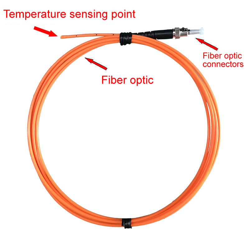
Sensor Layer – Fluorescent Fiber Optic Temperature Sensors
Fluorescent fiber optic sensors installed at each critical monitoring point provide MRI-compatible temperature measurement. Each sensor consists of:
- Miniature probe (1-3mm diameter, customizable) containing phosphorescent material
- Flexible optical fiber cable (0-80 meters length) transmitting excitation light and return fluorescence
- High-temperature adhesive or mechanical mounting securing sensor to monitored component
- Protective sleeving shielding fiber from mechanical damage
Key installation considerations:
- Route fiber cables through existing cable trays or conduits to transmitter location outside magnet room
- Maintain minimum bend radius (typically 25mm) preventing fiber breakage
- Label each fiber clearly at both sensor and transmitter ends ensuring proper channel assignment
- Verify sensor placement at actual hotspots using thermal imaging during installation validation
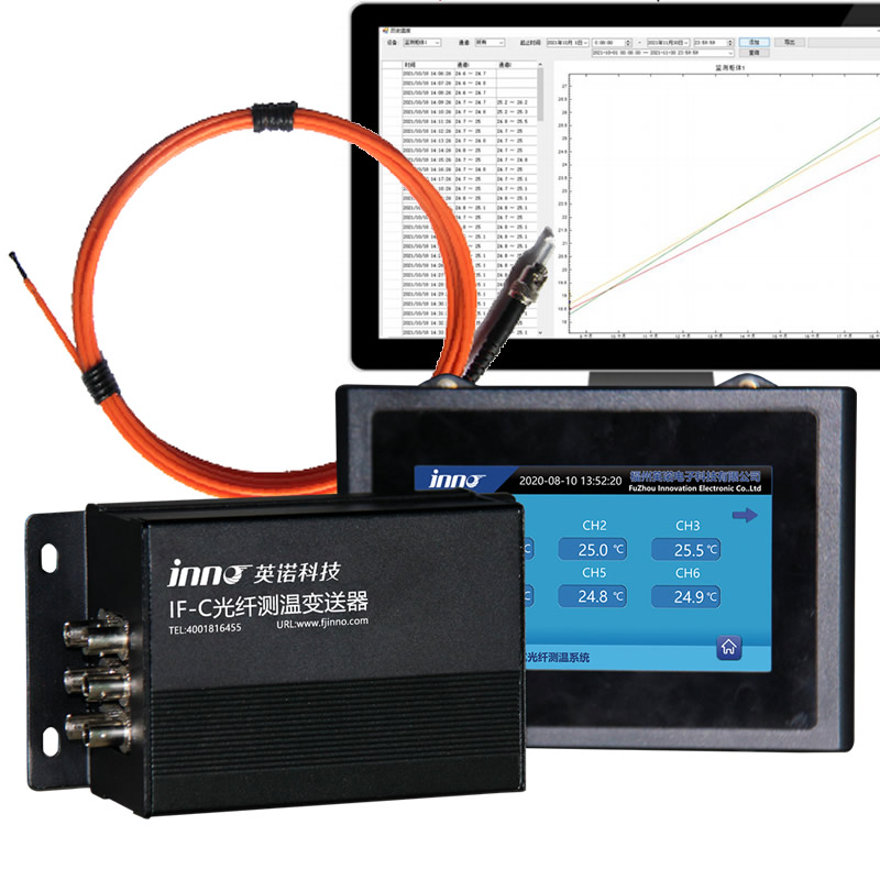
Data Acquisition Layer – Fiber Optic Temperature Transmitters
Fiber optic temperature transmitters convert optical signals to calibrated temperature readings. Modern transmitters offer:
- Multi-channel capacity – 1 to 64 independent channels, each measuring one specific hotspot via one dedicated fiber optic sensor
- High accuracy – ±1°C measurement accuracy across -40°C to +260°C range
- Fast response – <1 second measurement update rate enabling real-time monitoring
- Local display – Digital readout showing all channel temperatures for quick visual inspection
- Alarm outputs – Relay contacts or digital outputs triggering when thresholds exceeded
- Communication interfaces – Modbus RTU/TCP, Ethernet/IP, or analog outputs (4-20mA) for system integration
For a typical 3T MRI system, monitoring requirements might include:
- Gradient coils: 9 sensors (3 per axis at known hotspots)
- Gradient amplifiers: 6 sensors (2 per axis amplifier)
- RF power amplifier: 4 sensors
- Cooling system: 4 sensors (inlet, outlet, heat exchanger, reservoir)
- Equipment room: 4 sensors (ambient monitoring)
- Total: 27 sensors requiring one 32-channel transmitter
Communication Layer – Data Integration
Temperature data flows to multiple destinations:
- MRI console integration – Direct connection to scanner’s monitoring interface displaying temperatures alongside imaging parameters
- Facility SCADA – Integration with hospital building management systems via Modbus or BACnet protocols
- Service monitoring – Dedicated connection to manufacturer’s remote service platform for proactive support
- Local annunciator – Stack light or audible alarm in equipment room providing immediate operator notification
Management Layer – Analytics and Reporting
Centralized monitoring software provides:
- Real-time dashboards with graphical temperature trends and color-coded status
- Historical data logging with configurable retention periods (typically 1-5 years)
- Automated reporting for service documentation and regulatory compliance
- Predictive analytics identifying gradual degradation trends weeks before failures
- Correlation analysis linking temperature excursions to specific scan protocols or environmental conditions
Alarm Strategy Configuration
Multi-level temperature alarms enable graduated response preventing both nuisance alarms and catastrophic failures:
Gradient Coil Alarm Levels (Example)
- Pre-warning (60°C) – Logged notification, no operator action required, indicates cooling system may need attention during next maintenance
- Warning (65°C) – Operator notification, increased monitoring frequency, schedule service within 7 days
- High alarm (70°C) – Audible alarm, reduce scan intensity, avoid intensive sequences, schedule urgent service
- Critical alarm (75°C) – Automatic scan termination (if integration permits), immediate shutdown, emergency service contact
- Rate-of-rise alarm – Trigger if temperature increases >5°C in 5 minutes regardless of absolute value, indicating sudden cooling failure
Alarm Handling Protocols
Effective alarm management includes:
- Distinct alarm priorities preventing critical alarms from being obscured by routine notifications
- Automatic escalation if alarms remain unacknowledged (email to supervisor after 15 minutes, SMS to on-call engineer after 30 minutes)
- Contextual information with each alarm (affected component, temperature value, rate of change, recent history)
- Guided troubleshooting procedures accessed directly from alarm interface
Data Analytics Applications
Temperature trend analysis enables proactive maintenance:
Degradation Detection
Gradual temperature increase over weeks or months reveals cooling system degradation before critical failures. Example: Gradient coil outlet temperature rising from 18°C to 23°C over 6 months indicates heat exchanger fouling requiring cleaning.
Protocol Optimization
Comparing temperatures across different scan protocols identifies thermally stressful sequences. Research protocols can be modified to reduce gradient duty cycles while maintaining image quality, extending equipment life.
Environmental Correlation
Analyzing equipment temperatures versus ambient conditions validates HVAC performance and identifies seasonal variations requiring thermostat adjustments.
Predictive Maintenance Scheduling
Machine learning algorithms trained on historical temperature data predict component failures days or weeks in advance, enabling scheduled maintenance rather than emergency repairs.
Return on Investment
Comprehensive temperature monitoring delivers measurable value:
- Prevented failures – Early detection of cooling degradation prevents gradient coil damage ($150K-300K replacement cost)
- Reduced downtime – Scheduled maintenance during planned service windows rather than emergency repairs during clinical hours (potential revenue loss: $5K-15K per day)
- Extended equipment life – Maintaining optimal thermal conditions extends component service life 15-25%
- Improved patient safety – Preventing mid-scan shutdowns enhances patient experience and safety
Typical system investment: $15,000-30,000 for 30-40 monitoring points
Expected payback: 12-24 months through prevented failures and reduced downtime
11. Temperature Sensor Comparison: Why Fluorescent Fiber Optic Sensors
Selecting appropriate temperature sensing technology for MRI environments requires careful evaluation of competing technologies against the unique challenges of strong magnetic fields, radiofrequency interference, and space constraints.
Technology Principles
Fluorescent Fiber Optic Temperature Sensors
Fluorescent fiber optic sensors exploit temperature-dependent phosphorescent decay. A miniature probe tip contains rare-earth phosphor material (typically gadolinium oxysulfide or similar compounds) that fluoresces when excited by blue LED light transmitted through an optical fiber. The fluorescent decay time varies predictably with temperature from microseconds to milliseconds, providing accurate measurement completely independent of light intensity, fiber bending losses, or connector variations. These sensors provide contact-type measurement with one fiber optic cable measuring one specific hotspot location.
Resistance Temperature Detectors (RTDs)
PT100 sensors utilize platinum’s positive temperature coefficient (0.385Ω/°C per IEC 60751). A precisely wound platinum element with 100Ω resistance at 0°C changes resistance proportionally with temperature. Electronic transmitters convert resistance to temperature using standardized curves, achieving ±0.1°C accuracy under ideal conditions.
Thermocouples
Thermocouple sensors generate voltage from the Seebeck effect when junctions of dissimilar metals experience temperature differences. Type K (Chromel-Alumel) and Type T (Copper-Constantan) thermocouples are common for industrial applications, providing wide temperature ranges and fast response.
Infrared Thermometry
Infrared temperature measurement detects electromagnetic radiation (8-14μm wavelength) emitted by objects according to Stefan-Boltzmann law. Handheld infrared guns or fixed cameras calculate surface temperature from radiation intensity and material emissivity.
Comprehensive Performance Comparison
| Performance Parameter | Fluorescent Fiber Optic | PT100 RTD | Thermocouple | Infrared |
|---|---|---|---|---|
| Measurement Principle | Phosphorescent decay time | Resistance variation | Seebeck voltage | Thermal radiation |
| MRI Compatibility | Excellent (completely non-metallic) | Poor (requires special shielding) | Poor (metallic components) | Good (non-contact measurement) |
| Magnetic Field Immunity | Complete (no magnetic materials) | Susceptible to eddy currents | Susceptible to induced voltages | Not affected |
| RF Interference Immunity | Complete (optical transmission) | Highly susceptible without filters | Acts as antenna, severe interference | Not affected |
| Electrical Isolation | Inherent (dielectric fiber) | Requires galvanic isolation | Requires isolation amplifiers | Complete (non-contact) |
| Measurement Accuracy | ±1°C | ±0.3°C (Class A) to ±0.1°C (1/10 DIN) | ±1-2°C (Type K) to ±0.5°C (Type T) | ±2-5°C (emissivity dependent) |
| Temperature Range | -40°C to +260°C | -200°C to +850°C | -200°C to +1200°C (type dependent) | -20°C to +1500°C |
| Response Time | <1 second | 5-30 seconds (construction dependent) | 0.5-5 seconds (junction dependent) | <1 second |
| Probe Size | 1-3mm diameter (customizable) | 3-6mm typical | 0.5-3mm (wire type) to 6mm (probe) | N/A (spot size: 10-100mm typical) |
| Cable Length | 0-80 meters per sensor | Limited to 100m without compensation | Limited by wire resistance/noise | N/A (line-of-sight required) |
| Installation in MRI | Simple (adhesive mounting) | Very difficult (shielding required) | Very difficult (filtering required) | Requires viewing access |
| Gradient Coil Monitoring | Ideal (non-interfering, accurate) | Impractical (EMI, induced currents) | Impractical (severe interference) | Impossible (no viewing access) |
| Long-Term Stability | Excellent (no drift, >20 years) | Good (±0.1°C drift over 5 years) | Fair (junction degradation possible) | Depends on instrument calibration |
| Calibration Requirements | Factory calibrated, no field calibration | Periodic verification recommended | Periodic calibration required | Frequent calibration necessary |
| Multi-Point Capability | 1 hotspot per fiber, 1-64 channels per transmitter | One sensor per point, individual wiring | One junction per point, individual wiring | Thermal imaging of viewed area |
| Continuous Monitoring | Yes (24/7 real-time) | Yes (24/7 real-time) | Yes (24/7 real-time) | No (periodic surveys unless fixed) |
| Sensor Cost | $300-800 per point | $50-150 per sensor | $20-100 per sensor | $5,000-50,000 for camera system |
| Installation Cost (MRI) | Low (simple, no special requirements) | Very high (extensive shielding/filtering) | Very high (filtering, isolation) | Low (survey) to high (fixed camera) |
| Total System Cost (30 points) | $15,000-30,000 | $8,000-15,000 (non-MRI environment) | $5,000-10,000 (non-MRI environment) | $10,000-60,000 |
Why Fluorescent Fiber Optic Sensors Excel for MRI
Fluorescent fiber optic temperature sensors uniquely address the severe challenges of MRI environments that render conventional technologies impractical or impossible:
Complete MRI Compatibility
The total absence of metallic, magnetic, or conductive components eliminates all interactions with MRI’s magnetic fields and radiofrequency systems. Fiber optic sensors can be installed directly on gradient coils, inside RF shield rooms, or adjacent to the main magnet without affecting image quality, causing artifacts, or experiencing interference. This compatibility is absolutely critical—metallic sensors would create image artifacts, potentially becoming projectiles in the strong magnetic field, and suffering complete measurement failure from induced currents and RF interference.
Immunity to Electromagnetic Interference
MRI environments contain electromagnetic fields that would overwhelm electronic sensors:
- Static magnetic fields of 1.5-7 Tesla induce eddy currents in metallic sensor leads, creating measurement errors and heating
- Radiofrequency fields at 64-300 MHz (frequency dependent on field strength) couple into sensor wiring, saturating electronics
- Gradient switching at 200+ Hz creates time-varying magnetic fields inducing voltages of hundreds of volts in sensor loops
Optical fiber transmission completely eliminates these interference mechanisms. Temperature information travels as light pulses immune to all electromagnetic phenomena, ensuring accurate measurements even during intensive scanning protocols.
Intrinsic Electrical Safety
The dielectric nature of optical fibers provides absolute electrical isolation between monitored equipment and measurement instrumentation. This eliminates ground loop formation, prevents induced voltages from creating safety hazards, and allows monitoring of components at different electrical potentials without isolation amplifiers or barriers.
Installation Simplicity in Confined Spaces
Gradient coils, RF components, and cryogenic systems reside in extremely confined spaces within the MRI gantry. The small probe diameter (1-3mm, customizable) and flexible fiber optic cable enable installation in locations inaccessible to larger conventional sensors. Adhesive mounting or simple mechanical clips provide secure attachment without drilling, welding, or invasive procedures that might void equipment warranties.
Extended Transmission Distance Without Signal Degradation
Optical fiber cables transmit signals up to 80 meters with zero attenuation or noise addition. This capability allows centralized transmitter installation in equipment rooms while monitoring remote points deep within the magnet bore—impossible with conventional sensors requiring close proximity between sensor and electronics to minimize noise pickup.
Scalable Multi-Channel Architecture
A single fiber optic temperature transmitter accommodates 1-64 independent sensor channels, each providing dedicated measurement of one specific hotspot. This scalability enables comprehensive monitoring of an entire MRI system with minimal instrumentation:
- 9-12 gradient coil hotspots
- 6-8 gradient amplifier monitoring points
- 4-6 RF system locations
- 4-6 cooling system sensors
- 4-8 environmental monitoring points
- Total: 27-40 sensors served by one or two 32-channel transmitters
Maintenance-Free Long-Term Operation
The optical measurement principle exhibits exceptional stability with zero drift over decades of operation. Factory calibration remains valid for the sensor’s entire 20+ year lifespan, eliminating periodic calibration expenses and maintenance downtime. This longevity matches MRI equipment service life, avoiding sensor replacement during the scanner’s operational period.
Customizable Specifications for Diverse Requirements
Fluorescent fiber optic sensors offer customization addressing specific application needs:
- Temperature range – Standard -40°C to +260°C covers all MRI applications; extended ranges available for specialized equipment
- Probe diameter – Customizable from 1mm (ultra-compact) to 5mm (ruggedized) matching installation constraints
- Cable length – 0-80 meters accommodates any MRI facility layout
- Response time – <1 second standard; faster response possible for critical applications
- Accuracy – ±1°C standard; tighter tolerances achievable through calibration
Beyond MRI: Versatile Applications
While optimized for MRI environments, fluorescent fiber optic sensors excel across diverse applications sharing similar challenges:
Medical Equipment Monitoring
- CT scanners – X-ray tube and high-voltage generator temperature monitoring
- PET-CT systems – Detector module thermal management
- Linear accelerators – Radiation therapy system component monitoring
- Hyperbaric chambers – Patient monitoring in high-pressure, oxygen-rich environments where spark risk prohibits electronic sensors
Laboratory and Research Applications
- Cryogenic research – Temperature measurement in liquid nitrogen and liquid helium environments
- Microwave processing – Material heating in intense RF fields where metallic sensors would perturb the field or experience measurement errors
- Chemical reactors – Temperature monitoring in explosive atmospheres requiring intrinsically safe instrumentation
- Particle accelerators – Component monitoring in high-radiation environments
Industrial Process Monitoring
- Induction heating – Workpiece temperature measurement in strong magnetic fields
- RF drying systems – Material temperature during radiofrequency or microwave drying
- Transformer monitoring – Winding hotspot measurement in high-voltage environments
- Electric vehicle batteries – Cell-level thermal management without electromagnetic interference
Application-Specific Sensor Selection
While fluorescent fiber optic sensors provide optimal performance for MRI and electromagnetically harsh environments, sensor selection should match application requirements:
- Use fiber optic sensors whenever: MRI compatibility required, strong magnetic or RF fields present, electrical isolation critical, long transmission distances needed, maintenance-free operation desired
- Use PT100 sensors when: highest accuracy needed (±0.1°C), benign electromagnetic environment, established infrastructure for RTD transmitters exists
- Use thermocouples when: extremely high temperatures encountered (>500°C), fast response critical (microseconds), lowest cost prioritized in non-EMI environments
- Use infrared thermometry for: non-contact measurement requirements, thermal imaging surveys, rotating equipment, hazardous atmosphere monitoring
12. Medical Equipment Overview
Modern healthcare facilities deploy sophisticated medical imaging equipment and therapeutic systems requiring comprehensive temperature monitoring to ensure patient safety, diagnostic accuracy, and equipment reliability.
Diagnostic Imaging Systems
Magnetic Resonance Imaging (MRI)
As detailed throughout this guide, MRI scanners represent the most temperature-sensitive medical equipment due to cryogenic systems, high-power gradient and RF components, and sophisticated cooling requirements. Field strengths from 0.2T to 7T+ serve applications from routine orthopedic imaging to advanced neuroscience research.
Computed Tomography (CT) Scanners
CT systems utilize rotating X-ray tubes generating 60-120 kilowatts of heat during continuous scanning. Modern multi-detector CT scanners (64-320 slice configurations) demand aggressive cooling to prevent tube overheating that would interrupt cardiac or trauma imaging protocols. Temperature monitoring focuses on:
- X-ray tube anode temperature (critical limits: 1000-1500°C depending on design)
- X-ray generator components (high-voltage transformers, rectifiers)
- Cooling oil circulation system (typical operating range: 40-60°C)
- Detector array electronics (maintaining stable temperature for consistent calibration)
- Gantry bearing temperature (continuous rotation at 0.3-0.4 seconds per revolution)
Positron Emission Tomography (PET) Systems
PET scanners and integrated PET-CT systems incorporate temperature-sensitive scintillation crystal detector arrays. Temperature variations affect crystal light output and photomultiplier gain, degrading image quantitative accuracy critical for oncology treatment monitoring. Key monitoring points include:
- Detector module temperature (stability requirement: ±0.5°C for quantitative accuracy)
- Photomultiplier tube high-voltage supplies
- Electronics cooling system maintaining stable detector temperature despite ambient variations
- CT component cooling (for integrated PET-CT systems)
X-Ray Imaging Systems
Radiography, fluoroscopy, and angiography systems use high-power X-ray tubes requiring thermal monitoring:
- Tube anode temperature limiting consecutive exposures
- High-voltage generator component cooling
- Flat-panel detector temperature (affects noise and artifacts)
Ultrasound Systems
While generally less thermally demanding, advanced ultrasound systems with high-channel-count transducers and intensive Doppler processing benefit from monitoring:
- Transducer array temperature (piezoelectric element characteristics are temperature-dependent)
- Beamformer electronics in premium systems with 10,000+ channels
- Power supply and processor cooling
Radiation Therapy Equipment
Linear Accelerators (LINAC)
Linear accelerator systems for cancer radiotherapy generate multi-megawatt electron beams, creating intense thermal loads:
- Klystron or magnetron RF power sources (operating temperatures: 40-60°C)
- Accelerator waveguide structure (thermal expansion affects beam energy and stability)
- Bending magnet coils focusing and directing electron beam
- Multi-leaf collimator motors (100+ motorized leaves shaping radiation beam)
- Cooling water systems managing thermal loads exceeding 100 kilowatts
Proton Therapy Systems
Proton beam therapy facilities use superconducting or resistive magnets requiring extensive thermal management similar to MRI systems, plus high-power RF accelerating systems demanding temperature monitoring.
Laboratory and Analytical Equipment
Mass Spectrometers
Clinical laboratory mass spectrometry systems for toxicology, therapeutic drug monitoring, and newborn screening incorporate:
- Temperature-controlled ion sources maintaining reproducible ionization
- Vacuum pump cooling systems
- Electronics temperature stabilization for measurement consistency
Automated Chemistry Analyzers
High-throughput chemistry analyzers processing thousands of tests daily require precise temperature control:
- Reagent storage temperature (typically 4-8°C)
- Reaction chamber temperature (37°C ± 0.1°C for enzymatic assays)
- Sample storage temperature preventing degradation
- Optical detector temperature stability
Flow Cytometers
Flow cytometry systems for hematology and immunology incorporate temperature-sensitive lasers and detectors requiring stable thermal environments.
Surgical and Interventional Equipment
Surgical Lasers
Medical laser systems (CO₂, Nd:YAG, diode lasers) generate significant heat requiring active cooling:
- Laser cavity or diode array temperature
- Power supply cooling (particularly for high-power surgical lasers)
- Delivery system components (fiber optic transmission generates heat from optical losses)
Radiofrequency Ablation Systems
RF ablation generators for tumor treatment and cardiac arrhythmia therapy deliver 50-200 watts, requiring temperature monitoring at:
- Generator power stage components
- Ablation catheter tip temperature (directly affects tissue heating)
- Cooling pump system maintaining catheter tip temperature
Cryotherapy Systems
Cryoablation equipment creates extreme cold (-40°C to -160°C) for tumor destruction, requiring temperature monitoring ensuring adequate freeze zone creation and equipment safety.
Life Support and Critical Care Equipment
Extracorporeal Membrane Oxygenation (ECMO)
ECMO systems providing cardiac and respiratory support incorporate heater-cooler units requiring precise temperature control (typically 36-37°C blood temperature) with continuous monitoring preventing patient thermal injury.
Hypothermia/Hyperthermia Systems
Therapeutic temperature management systems for cardiac arrest, stroke, and neurosurgical procedures require accurate body temperature monitoring via esophageal or bladder temperature probes.
Sterilization and Decontamination
Steam Sterilizers (Autoclaves)
Sterilization equipment processes surgical instruments at 121-134°C requiring validated temperature monitoring demonstrating adequate sterilization conditions throughout the load.
Low-Temperature Sterilization
Hydrogen peroxide plasma and ethylene oxide sterilizers for temperature-sensitive instruments require chamber temperature monitoring ensuring optimal sterilant efficacy.
13. Fiber Optic Temperature Monitoring for Equipment Hotspot Detection
Fiber optic temperature monitoring systems provide comprehensive thermal surveillance across medical equipment, detecting developing problems before they cause failures, ensuring patient safety, and optimizing maintenance strategies.
MRI System Comprehensive Monitoring
Gradient Coil Monitoring Implementation
Gradient coil temperature monitoring represents the highest-priority application preventing the most common MRI thermal failure mode. Optimal implementation includes:
Sensor Placement Strategy:
- X-gradient coil – 3-4 sensors at known hotspots identified during factory testing (typically coil center and ends where current density peaks)
- Y-gradient coil – 3-4 sensors at corresponding locations
- Z-gradient coil – 2-3 sensors (often generates less heat than transverse gradients)
- Cooling manifolds – 2-3 sensors on water inlet/outlet measuring cooling effectiveness
- Total: 10-14 sensors for comprehensive gradient system coverage
Installation Procedure:
- Access gradient coil assembly (typically requires partial bore disassembly)
- Clean mounting surfaces with alcohol removing oils and contaminants
- Apply high-temperature adhesive (rated >150°C) to sensor probe
- Press sensor firmly against coil surface at predetermined location, holding 30-60 seconds for initial cure
- Allow 24-hour full cure before energizing gradient system
- Route fiber optic cables through existing cable trays to equipment room
- Connect fibers to transmitter channels, documenting location of each sensor
- Verify all channels report plausible temperatures (ambient ±5°C before energizing system)
- Establish baseline temperatures during typical scan protocols
- Configure alarm thresholds based on manufacturer specifications and baseline data
Case Study: Research MRI Gradient Monitoring
A university hospital operating a 7T research MRI scanner for brain connectivity studies experienced frequent thermal shutdowns interrupting 2-hour research protocols. Installation of 12 fluorescent fiber optic sensors on gradient coils revealed asymmetric heating—Y-gradient reaching 78°C while X and Z gradients remained at 58-62°C. Investigation discovered partially blocked cooling channel in Y-gradient coil. After clearing the obstruction, Y-gradient temperature decreased to 54-60°C, eliminating shutdowns and enabling completion of research studies. The monitoring system paid for itself within three weeks by preventing research protocol failures and maintaining study participant enrollment.
RF System Temperature Monitoring
RF power amplifier monitoring prevents expensive component failures:
- Power transistor heat sinks – 2-4 sensors per amplifier stage monitoring junction temperature indirectly
- Amplifier enclosure – Ambient temperature inside electronics bay
- Cooling airflow – Temperature differential between inlet and outlet air indicating heat removal rate
- Body coil connections – Interface points where RF power couples into body coil
Multi-channel receiver coils with local preamplifiers benefit from element-level monitoring:
- Preamplifier temperature in high-density arrays (32-128 elements)
- Detuning circuit components that may overheat during transmit pulses
- Cable shield currents manifesting as localized heating at specific points
Cryogenic System Monitoring
Beyond helium level monitoring, temperature surveillance provides early warning of cryogenic system degradation:
- Cold head stage temperatures – First stage should maintain 40-50K, second stage 4-5K; deviations indicate compressor issues
- Thermal shield temperatures – Multiple sensors around circumference detect vacuum degradation or radiation shield damage
- Outer vessel temperature – Should remain near ambient; elevated readings suggest vacuum loss
- Penetration points – Current leads, instrumentation wires, and fill ports represent thermal leaks requiring monitoring
CT Scanner Temperature Monitoring
X-Ray Tube Thermal Management
CT X-ray tubes represent the most expensive consumable component ($200K-500K replacement cost). Temperature monitoring extends tube life:
- Anode temperature measurement – Direct measurement via fiber optic sensors embedded in anode structure during manufacturing provides accurate data for dynamic scan protocol adjustment
- Bearing temperature – Elevated bearing temperature (normally 40-60°C) indicates lubrication degradation or mechanical wear
- Cooling oil temperature – Inlet and outlet temperatures with differential indicating heat removal effectiveness
- Tube housing temperature – Excessive housing temperature suggests cooling oil circulation problems
Implementation Benefits:
- Dynamic tube loading optimization – Adjust scan parameters in real-time based on actual thermal state rather than conservative estimates
- Predictive tube replacement – Schedule tube changes based on thermal degradation indicators rather than unexpected failures
- Scan throughput optimization – Maximize consecutive scans while maintaining safe thermal margins
Generator and Power Electronics
High-voltage generator components handling 100+ kW require thermal monitoring:
- High-voltage transformer temperature (oil-filled or cast resin types)
- Rectifier and capacitor bank temperatures
- Inverter IGBT junction temperatures
- Cooling system heat exchanger effectiveness
PET-CT System Monitoring
Detector Temperature Stabilization
PET detector modules require ±0.5°C stability for quantitative imaging accuracy:
- Crystal array temperature – Direct measurement of scintillation crystal temperature affecting light output
- Photomultiplier tube temperature – PMT gain varies significantly with temperature (~0.2-0.5% per °C)
- Cooling system performance – Verify active temperature control maintains setpoint despite ambient variations
- Electronics board temperature – Signal processing electronics affecting timing resolution and energy discrimination
Maintaining detector temperature stability ensures:
- Quantitative SUV (Standardized Uptake Value) accuracy for oncology treatment response assessment
- Consistent image quality across different ambient conditions and scanner utilization patterns
- Reduced calibration frequency requirements
Linear Accelerator Monitoring
RF Power System Temperature Tracking
LINAC RF systems generating multi-megawatt pulses require comprehensive thermal monitoring:
- Klystron or magnetron temperature – Tube body and collector cooling
- Modulator components – Pulse-forming network, switching tubes, transformers
- Circulator and load – Components absorbing reflected RF power
- Waveguide components – Critical sections that may develop standing wave heating
Beam Transport and Delivery
Temperature monitoring ensures beam stability and safety:
- Bending magnet coils – Resistive magnets generating significant heat
- Beam target – Electron beam striking tungsten target generates intense local heating
- Multi-leaf collimator motors – 120+ motors shaping radiation field, each generating heat
- Gantry bearings – Continuous rotation of multi-ton gantry creates bearing heat
Monitoring System Architecture for Multiple Equipment
Large medical facilities with diverse equipment fleets benefit from integrated temperature monitoring infrastructure:
| Equipment Type | Critical Monitoring Points | Sensors per Unit | Typical Fleet Size | Total Sensors |
|---|---|---|---|---|
| 3T MRI | Gradients, RF, cryogenics, cooling | 24-32 | 2-3 units | 48-96 |
| 1.5T MRI | Gradients, RF, cryogenics, cooling | 20-28 | 3-5 units | 60-140 |
| CT Scanners | X-ray tube, generator, cooling | 8-12 | 4-6 units | 32-72 |
| PET-CT | Detectors, CT components | 16-24 | 1-2 units | 16-48 |
| Linear Accelerators | RF system, magnets, MLC, gantry | 12-20 | 2-4 units | 24-80 |
| Environmental | Equipment rooms, magnet rooms | 4-8 per room | 10-15 rooms | 40-120 |
| Total System | 220-556 sensors | |||
This monitoring point count typically requires 8-12 fiber optic temperature transmitters (64-channel models) with centralized monitoring software providing:
- Unified dashboard displaying all equipment thermal status
- Cross-system correlation identifying facility-wide issues (HVAC failures affecting multiple systems)
- Integrated alarm management with intelligent routing to appropriate personnel
- Comprehensive reporting for regulatory compliance and accreditation
- Predictive analytics identifying systemic degradation patterns
Success Metrics and ROI
Healthcare organizations implementing comprehensive fiber optic temperature monitoring across imaging equipment report:
- Equipment uptime improvement – 3-5% increase in availability through predictive maintenance (for a $2M MRI performing 6000 studies annually at $800 average reimbursement = $144K-240K additional revenue)
- Component life extension – 20-30% longer X-ray tube life in CT scanners ($50K-150K savings per tube), 15-25% gradient coil life extension in MRI ($45K-75K annual savings per scanner)
- Emergency repair reduction – 60-70% fewer emergency service calls (typical emergency service: $5K-15K vs. planned maintenance: $2K-4K)
- Patient satisfaction – Reduced mid-scan interruptions from thermal shutdowns improving patient experience scores
- Regulatory compliance – Simplified documentation for Joint Commission, state health department, and accreditation body inspections
Typical 5-year ROI calculation for major medical center:
- Initial investment: $150,000 (300 monitoring points across 15 major systems)
- Annual prevented failures: $200,000 (4-5 major component failures avoided)
- Annual increased revenue: $300,000 (improved uptime on high-value equipment)
- Annual reduced emergency repairs: $80,000
- Total 5-year benefit: $2,900,000
- Net ROI: 1,833% over 5 years
14. Frequently Asked Questions
Q1: How long does an MRI system typically last?
A: Properly maintained MRI scanners provide 15-20 years of clinical service before technological obsolescence or major system upgrades become necessary. The superconducting magnet itself can function 30+ years—some magnets from 1980s installations remain operational today. However, gradient systems, RF components, and computer systems typically require replacement or major upgrades at 10-15 year intervals. Comprehensive temperature monitoring extends component life by preventing thermal damage, often achieving 20-25% longer service from gradient coils and RF amplifiers.
Q2: How often must helium be refilled in MRI systems?
A: Modern MRI cryogenic systems with zero-boil-off technology require helium refills every 3-5 years under normal conditions, compared to annual or more frequent refills in older designs. The two-stage cold head compressor re-liquefies evaporated helium, reducing boil-off rates from historical 2-5 liters/day to current 0.1-0.5 liters/day. However, cold head compressor failure, vacuum degradation, or magnet quench events may necessitate emergency refills. Helium costs fluctuate significantly ($10-40 per liter depending on market conditions), making a typical 800-1200 liter refill cost $8,000-48,000.
Q3: What are the temperature and humidity requirements for MRI rooms?
A: MRI magnet rooms require environmental control maintaining 18-22°C (64-72°F) temperature with ±2°C maximum variation and 30-60% relative humidity. These specifications ensure gradient coil and RF system cooling effectiveness, prevent condensation on cold surfaces, and maintain consistent imaging performance. Equipment rooms housing gradient amplifiers and RF power systems require similar temperature control, often with tighter limits (20°C ±1°C) due to higher heat dissipation. HVAC systems must handle 30-50 kilowatts total heat load from the complete MRI installation. Temperature excursions above 25°C significantly reduce thermal margin, potentially causing gradient overheating and scan interruptions.
Q4: Why do MRI systems need special temperature sensors?
A: MRI environments create unique challenges that render conventional temperature sensors impractical or impossible to use. The strong static magnetic field (1.5-7 Tesla) induces eddy currents in metallic sensor components, creating measurement errors and dangerous heating. Radiofrequency pulses (64-300 MHz) couple into sensor wiring, saturating electronics and causing severe interference. Rapid gradient switching generates time-varying magnetic fields inducing hundreds of volts in sensor loops. Fluorescent fiber optic temperature sensors solve these problems through completely non-metallic, non-conductive construction that is immune to all electromagnetic phenomena while providing accurate temperature measurement.
Q5: What causes MRI magnet quenches and how can they be prevented?
A: Magnet quench events—sudden loss of superconductivity—occur when superconducting wire temperature rises above the critical threshold (~10 Kelvin). Common causes include: ferromagnetic object impacts disturbing magnet winding alignment, cold head compressor failure allowing helium temperature rise, vacuum degradation in cryostat insulation increasing heat load, or mechanical disturbances from earthquakes. Prevention strategies include: maintaining cold head compressor operation through regular service (15,000-20,000 hour intervals), continuous helium level and temperature monitoring with early warning alarms, strict ferromagnetic object screening preventing projectile accidents, periodic vacuum monitoring detecting insulation degradation, and seismic protection in earthquake-prone regions. While quenches rarely cause permanent damage, the $20K-40K helium refill cost and 1-2 week recovery time make prevention critical.
Q6: Why do gradient coils overheat?
A: Gradient coil overheating results from the fundamental conflict between imaging performance demands and thermal limits. Fast imaging sequences like echo-planar imaging (EPI) for diffusion or functional MRI switch gradients at maximum amplitude 200+ times per second, dissipating 30-50 kilowatts. Contributing factors include: cooling system degradation from pump wear or heat exchanger fouling reducing heat removal capacity 20-40%, intensive scanning protocols (research studies) running at maximum duty cycles for extended periods, elevated ambient temperature from HVAC failures reducing thermal margin, and sequential intensive scans without adequate cool-down intervals. Continuous temperature monitoring with fluorescent fiber optic sensors provides early warning enabling cooling system maintenance, scan protocol optimization, or forced cool-down periods before reaching critical temperatures.
Q7: How difficult is it to install fiber optic temperature sensors in MRI systems?
A: Fluorescent fiber optic sensor installation is straightforward compared to conventional sensor technologies. The process involves: accessing gradient coil assembly or RF components (typically 2-4 hours for bore disassembly), cleaning sensor mounting locations with alcohol, applying high-temperature adhesive to miniature sensor probes (1-3mm diameter), pressing sensors onto monitored surfaces, routing flexible fiber optic cables (0.5-2mm diameter) through existing cable trays to equipment room (1-2 hours), connecting fibers to transmitter channels (15-30 minutes), and verifying all measurements (30 minutes). Total installation time for 24-32 monitoring points: 6-10 hours including system access and reassembly. The non-metallic sensor construction eliminates complex grounding schemes, shielding requirements, or filtering needed for electronic sensors, significantly simplifying installation.
Q8: What is the typical cost for MRI temperature monitoring systems?
A: Comprehensive MRI temperature monitoring systems cost $20,000-35,000 for a complete installation monitoring 24-32 critical points including gradient coils, RF systems, cooling circuits, and environmental conditions. This includes: fluorescent fiber optic sensors ($300-600 each), fiber optic temperature transmitter(s) ($8,000-15,000 for 32-64 channels), installation labor ($3,000-6,000), system configuration and commissioning ($2,000-4,000), and monitoring software ($2,000-5,000). For multi-scanner facilities, per-system costs decrease 20-30% through economies of scale. Return on investment typically occurs within 12-24 months through prevented gradient coil failures ($150K-300K replacement cost), avoided emergency service calls ($5K-15K per incident), and increased scanner utilization from reduced downtime. The investment represents 0.7-1.2% of typical MRI system cost while providing disproportionate value in risk reduction.
Q9: How many sensor channels can one fiber optic transmitter support?
A: Fiber optic temperature transmitters are available in configurations supporting 1 to 64 independent channels, with each channel connecting to one dedicated fluorescent sensor measuring one specific hotspot location. Common configurations include 4, 8, 16, 32, and 64-channel models. A single MRI scanner typically requires 24-32 monitoring points (gradient coils, RF components, cooling system, environment), well-served by one 32-channel or 64-channel transmitter. Multi-scanner facilities benefit from centralized monitoring using one or two large transmitters (64-channel models) serving 40-80+ sensors across multiple systems. The contact-type measurement principle means one fiber optic cable measures one hotspot—not distributed multi-point sensing. Modular transmitter designs allow field expansion as monitoring needs grow.
Q10: Can the same fiber optic sensors monitor other medical equipment besides MRI?
A: Absolutely. Fluorescent fiber optic temperature sensors provide versatile monitoring across all medical equipment where accurate temperature measurement is critical. Applications beyond MRI include: CT scanner X-ray tubes and generators (electromagnetic compatibility important), PET-CT systems requiring detector temperature stabilization (±0.5°C accuracy), linear accelerators for radiation therapy (RF power systems, magnets, motors), surgical lasers and RF ablation systems (high-power electronics monitoring), automated laboratory analyzers (reaction chambers, reagent storage), ECMO and cardiopulmonary bypass systems (patient temperature monitoring), and sterilization equipment (process validation). The sensors’ customizable specifications (temperature range, probe size, cable length, response time) enable tailored solutions for virtually any medical equipment temperature monitoring requirement.
Q11: How does temperature monitoring integrate with hospital information systems?
A: Modern fiber optic temperature transmitters provide industry-standard communication protocols enabling seamless integration with hospital infrastructure. Common interfaces include: Modbus RTU/TCP for building management systems and equipment monitoring networks, BACnet for HVAC and facility automation platforms, Ethernet/IP or PROFINET for industrial control systems, SNMP for network management and alarm distribution, and OPC UA for enterprise-level data integration. Analog outputs (4-20mA) and relay contacts provide direct connection to legacy systems. Integration typically involves configuring transmitter IP address and register mapping (1-2 hours), adding monitoring points to SCADA or building automation database (2-4 hours), and configuring alarm routing to email, SMS, or paging systems (1-2 hours). Most installations complete within one day. Data can flow to: biomedical engineering management systems, computerized maintenance management systems (CMMS), and enterprise asset management platforms supporting predictive maintenance strategies.
Q12: What temperature range can fluorescent fiber optic sensors measure?
A: Standard fluorescent fiber optic temperature sensors measure from -40°C to +260°C, covering all MRI and medical equipment applications from cryogenic monitoring to high-temperature sterilization processes. This range accommodates: gradient coil monitoring (typical operation 35-70°C, critical alarms 75-85°C), RF amplifier monitoring (40-90°C operating range), cryogenic cold head monitoring (-269°C to 80K, though specialized sensors required below -40°C), CT X-ray tube monitoring (anode temperatures up to 1500°C require different sensor technology, but associated components 40-120°C), sterilizer chamber monitoring (121-134°C steam sterilization), and environmental monitoring (room temperatures 15-30°C). The -40°C to +260°C range provides substantial margin above typical medical equipment operating temperatures while the ±1°C accuracy specification ensures reliable detection of abnormal thermal conditions.
Q13: Are fluorescent fiber optic sensors’ specifications customizable?
A: Yes, fluorescent fiber optic temperature sensors offer extensive customization matching specific application requirements. Customizable parameters include: Temperature range – Standard -40°C to +260°C; extended ranges available for specialized applications (cryogenic to +400°C for industrial processes); Measurement accuracy – Standard ±1°C; tighter tolerances achievable (±0.5°C or better through individual calibration); Probe diameter – Standard 1-3mm; customizable from 0.5mm (ultra-miniature for confined spaces) to 6mm (ruggedized for harsh environments); Probe length – 10mm to 100mm+ depending on thermal mass and response time requirements; Fiber cable length – 0.5 to 80 meters standard; longer distances possible with specialized configurations; Response time – Standard <1 second; faster response achievable with reduced probe thermal mass; Cable jacket – Standard PVC; Teflon, stainless steel, or armored options for chemical resistance or mechanical protection. Consult with sensor manufacturers to specify optimal configuration for each unique monitoring application.
Q14: What happens if a fiber optic temperature sensor fails?
A: Fiber optic sensor failures are rare (failure rate <0.1% annually) due to robust optical measurement principles and absence of electrical components subject to degradation. When failures occur, they typically result from: mechanical fiber breakage from excessive bending or impact (most common), adhesive failure causing sensor detachment from monitored surface, or connector damage at transmitter interface. The transmitter immediately detects sensor failure through loss of optical signal and generates a sensor fault alarm indicating the affected channel. Critically, all other sensors continue operating normally—unlike distributed systems where single fiber break disables multiple measurement points. Sensor replacement involves: disconnecting the failed fiber at the transmitter (30 seconds), accessing the monitored component (time varies by location: 5 minutes for accessible points, 2-4 hours for internal MRI components), removing the failed sensor, installing a new sensor with fresh adhesive, routing the new fiber to the transmitter, connecting to the same channel number (maintaining documentation consistency), and verifying proper operation (5 minutes). Total replacement time: 15-30 minutes for accessible locations, 3-5 hours for internal MRI locations requiring system disassembly.
Q15: How does continuous temperature monitoring extend MRI equipment lifespan?
A: Comprehensive temperature monitoring extends MRI component and system lifespan through multiple mechanisms. Gradient coil protection – Preventing overheating episodes that cause epoxy delamination, coil deformation, and insulation degradation extends coil life from typical 12-15 years to 18-20 years (replacement cost avoided: $150K-300K). RF system preservation – Maintaining amplifier components within thermal specifications prevents premature transistor and capacitor failures, extending amplifier life 20-30%. Cooling system optimization – Early detection of heat exchanger fouling or pump degradation enables preventive maintenance before catastrophic failures damage multiple subsystems. Cryogenic system protection – Cold head monitoring prevents helium boil-off rate increases that accelerate cryogen depletion (refill cost: $20K-40K). Environmental control – Verifying proper room temperature prevents thermal stress on all components simultaneously. The cumulative effect: comprehensive monitoring extends overall MRI system productive lifespan 15-25%, deferring capital replacement costs ($1.5M-3M+ for new scanner) by 3-5 years while maintaining clinical image quality and reliability throughout the extended service period.
Get Expert MRI Temperature Monitoring Solutions
Contact us today for customized temperature monitoring solutions for your medical imaging equipment.

Fiber optic temperature sensor, Intelligent monitoring system, Distributed fiber optic manufacturer in China
 |
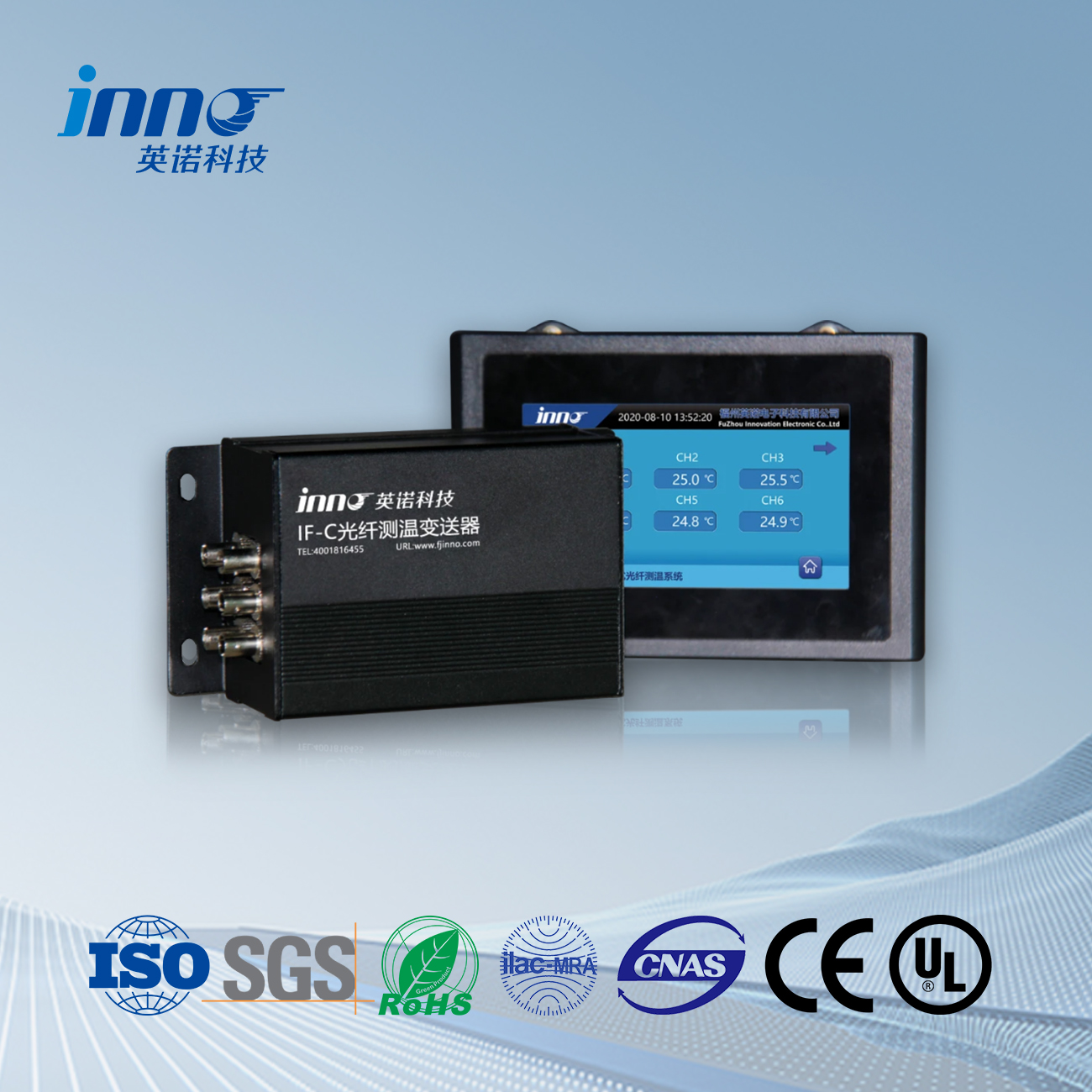 |
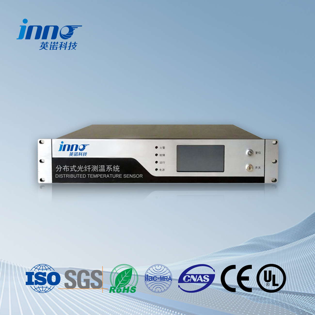 |